ATaCR
Introduction
atacr is a module for the correction of vertical component data from OBS
stations from tilt and compliance noise. This module is a translation of the
Matlab code ATaCR and the acronym
stands for Automatic Tilt and Compliance Removal. For more details on the
theory and methodology, we refer the interested reader to the following papers:
Bell, S. W., D. W. Forsyth, and Y. Ruan (2014), Removing noise from the vertical component records of ocean-bottom seismometers: Results from year one of the Cascadia Initiative, Bull. Seismol. Soc. Am., 105, 300-313, https://doi.org/10.1785/0120140054
Crawford, W.C., Webb, S.C., (2000). Identifying and removing tilt noise from low-frequency (0.1 Hz) seafloor vertical seismic data, Bull. seism. Soc. Am., 90, 952-963, https://doi.org/10.1785/0119990121
Janiszewski, H A, J B Gaherty, G A Abers, H Gao, Z C Eilon, Amphibious surface-wave phase-velocity measurements of the Cascadia subduction zone, Geophysical Journal International, Volume 217, Issue 3, June 2019, Pages 1929-1948, https://doi.org/10.1093/gji/ggz051
The analysis can be carried out for either one (or both) compliance or tilt corrections. In all cases the analysis requires at least vertical component data. Additional data required depend on the type of analysis. The software will automatically calculate all possible corrections depending on the available channels.
Noise Corrections
Compliance
Compliance is defined as the spectral ratio between pressure and vertical
displacement data. Compliance noise arises from seafloor deformation due
to seafloor and water wave effects (including infragravity waves).
This is likely the main source of noise in vertical component OBS data.
This analysis therefore requires both vertical (?HZ) and pressure (?DH) data.
Tilt
Tilt noise arises from OBS stations that are not perfectly leveled, and
therefore the horizontal seafloor deformation leaks onto the vertical
component. This effect can be removed by calculating the spectral
ratio between horizontal and vertical displacement data. In most cases,
however, the tilt direction (measured on a compass - as opposed to tilt
angle, measured from the vertical axis) is unknown and must be determined
from the coherence between rotated horizontal components and the vertical
component. This analysis therefore requires vertical (?HZ) and the two
horizontal (?H1,2) component data.
Compliance + Tilt
It is of course possible to combine both corrections and apply them
sequentially. In this case the tilt noise is removed first, followed by compliance.
This analysis requires all four components: three-component
seismic (?HZ,1,2) and pressure (?DH) data.
API documentation
Base Classes
atacr defines the following base classes:
The class DayNoise contains attributes
and methods for the analysis of two- to four-component day-long time-series
(3-component seismograms and pressure data). Objects created with this class
are required in any subsequent analysis. The available methods calculate the
power-spectral density (PSD) functions of sub-windows (default is 2-hour windows)
and identifies windows with anomalous PSD properties. These windows are flagged
and are excluded from the final averages of all possible PSD and cross-spectral density
functions between all available components.
The class StaNoise contains attributes
and methods for the aggregation of averaged daily spectra into a station
average. An object created with this class requires that at least two
DayNoise objects are available in memory. Methods available for this class are
similar to those defined in the DayNoise class, but are applied to daily
spectral averages, as opposed to sub-daily averages. The result is a spectral
average that represents all available data for the specific station.
The class TFNoise contains attributes
and methods for the calculation of transfer functions from noise
traces used to correct the vertical component. A TFNoise object works with
either one of DayNoise and StaNoise objects to calculate all possible
transfer functions across all available components. These transfer functions
are saved as attributes of the object in a Dictionary.
The class EventStream contains attributes
and methods for the application of the transfer functions to the
event traces for the correction (cleaning) of vertical component
seismograms. An EventStream object is initialized with raw (or pre-processed)
seismic and/or pressure data and needs to be processed using the same (sub) window
properties as the DayNoise objects. This ensures that the component corrections
are safely applied to produce corrected (cleaned) vertical components.
atacr further defines the following container classes:
These classes are used as containers for individual traces/objects that are used as attributes of the base classes.
Note
In the examples below, the SAC data were obtained and pre-processed
using the accompanying scripts atacr_download_data and
atacr_download_event. See the script and tutorial for details.
DayNoise
- class obstools.atacr.classes.DayNoise(tr1=None, tr2=None, trZ=None, trP=None, window=7200.0, overlap=0.3, key='')[source]
A DayNoise object contains attributes that associate three-component raw (or deconvolved) traces, metadata information and window parameters. The available methods carry out the quality control steps and the average daily spectra for windows flagged as “good”.
Note
The object is initialized with
Traceobjects for H1, H2, HZ and P components. Traces can be empty if data are not available. Upon saving, those traces are discarded to save disk space.- tr1, tr2, trZ, trP
Corresponding trace objects for components H1, H2, HZ and HP. Traces can be empty (i.e.,
Trace()) for missing components.- Type:
Traceobject
- window
Length of time window in seconds
- Type:
float
- overlap
Fraction of overlap between adjacent windows
- Type:
float
- key
Station key for current object
- Type:
str
- dt
Sampling distance in seconds. Obtained from
trZobject- Type:
float
- npts
Number of points in time series. Obtained from
trZobject- Type:
int
- fs
Sampling frequency (in Hz). Obtained from
trZobject- Type:
float
- year
Year for current object (obtained from UTCDateTime). Obtained from
trZobject- Type:
str
- julday
Julian day for current object (obtained from UTCDateTime). Obtained from
trZobject- Type:
str
- ncomp
Number of available components (either 2, 3 or 4). Obtained from non-empty
Traceobjects- Type:
int
- tf_list
Dictionary of possible transfer functions given the available components.
- Type:
Dict
Examples
Get demo noise data as DayNoise object
>>> from obstools.atacr import DayNoise
>>> daynoise = DayNoise('demo')
Uploading demo data - March 04, 2012, station 7D.M08A
Now check its main attributes
>>> print(*[daynoise.tr1, daynoise.tr2, daynoise.trZ, daynoise.trP], sep="\n")
7D.M08A..BH1 | 2012-03-04T00:00:00.000000Z - 2012-03-04T23:59:59.800000Z | 5.0 Hz, 432000 samples
7D.M08A..BH2 | 2012-03-04T00:00:00.000000Z - 2012-03-04T23:59:59.800000Z | 5.0 Hz, 432000 samples
7D.M08A..BHZ | 2012-03-04T00:00:00.000000Z - 2012-03-04T23:59:59.800000Z | 5.0 Hz, 432000 samples
7D.M08A..BDH | 2012-03-04T00:00:00.000000Z - 2012-03-04T23:59:59.800000Z | 5.0 Hz, 432000 samples
>>> daynoise.window
7200.0
>>> daynoise.overlap
0.3
>>> daynoise.key
'7D.M08A'
>>> daynoise.ncomp
4
>>> daynoise.tf_list
{'ZP': True, 'Z1': True, 'Z2-1': True, 'ZP-21': True, 'ZH': True, 'ZP-H': True}
- QC_daily_spectra(pd=[0.004, 0.2], tol=1.5, alpha=0.05, smooth=True, fig_QC=False, debug=False, save=None, form='png')[source]
Method to determine daily time windows for which the spectra are anomalous and should be discarded in the calculation of the transfer functions.
- Parameters:
pd (list) – Frequency corners of passband for calculating the spectra
tol (float) – Tolerance threshold. If spectrum > std*tol, window is flagged as bad
alpha (float) – Confidence interval for f-test
smooth (boolean) – Determines if the smoothed (True) or raw (False) spectra are used
fig_QC (boolean) – Whether or not to produce a figure showing the results of the quality control
debug (boolean) – Whether or not to plot intermediate steps in the QC procedure for debugging
save (
Pathobject) – Relative path to figures folderform (str) – File format (e.g., ‘png’, ‘jpg’, ‘eps’)
- ftX
Windowed Fourier transform for the X component (can be either 1, 2, Z or P)
- Type:
ndarray
- f
Full frequency axis (Hz)
- Type:
ndarray
- goodwins
List of booleans representing whether a window is good (True) or not (False)
- Type:
list
Examples
Perform QC on DayNoise object using default values and plot final figure
>>> from obstools.atacr import DayNoise
>>> daynoise = DayNoise('demo')
Uploading demo data - March 04, 2012, station 7D.M08A
>>> daynoise.QC_daily_spectra(fig_QC=True)
Print out new attribute of DayNoise object
>>> daynoise.goodwins
array([False,  True,  True,  True,  True,  True,  True,  True, False,
   False,  True,  True,  True,  True,  True,  True], dtype=bool)
- average_daily_spectra(calc_rotation=True, tiltfreqs=[0.005, 0.035], fig_average=False, fig_tilt=False, save=None, form='png')[source]
Method to average the daily spectra for good windows. By default, the method will attempt to calculate the tilt orientation from the maximum coherence between component H1 and the vertical component HZ and use the rotated horizontals in the transfer function calculations for tilt noise removal.
- Parameters:
calc_rotation (boolean) – Whether or not to calculate the tilt direction
tiltfreqs (list) – Two floats representing the frequency band at which the tilt is calculated
fig_average (boolean) – Whether or not to produce a figure showing the average daily spectra
fig_tilt (boolean) – Whether or not to produce a figure showing the maximum coherence and phase between H1 and HZ as function of azimuth measured CW from H1, and the spectra for these components
save (
Pathobject) – Relative path to figures folderform (str) – File format (e.g., ‘png’, ‘jpg’, ‘eps’)
Examples
Average spectra for good windows using default values and plot final figure
>>> from obstools.atacr import DayNoise
>>> daynoise = DayNoise('demo')
Uploading demo data - March 04, 2012, station 7D.M08A
>>> daynoise.QC_daily_spectra()
>>> daynoise.average_daily_spectra(fig_average=True)
Print out available attributes of DayNoise object
>>> daynoise.__dict__.keys()
dict_keys(['tr1', 'tr2', 'trZ', 'trP', 'window', 'overlap', 'key',
'dt', 'npts', 'fs', 'year', 'julday', 'tkey', 'ncomp', 'tf_list',
'QC', 'av', 'f', 'goodwins', 'power', 'cross', 'rotation'])
- save(filename)[source]
Method to save the object to file using ~Pickle.
- Parameters:
filename (str) – File name
Examples
Run demo through all methods
>>> from obstools.atacr import DayNoise
>>> daynoise = DayNoise('demo')
Uploading demo data - March 04, 2012, station 7D.M08A
>>> daynoise.QC_daily_spectra()
>>> daynoise.average_daily_spectra()
Save object
>>> daynoise.save('daynoise_demo.pkl')
Check that it has been saved
>>> import glob
>>> glob.glob("./daynoise_demo.pkl")
['./daynoise_demo.pkl']
StaNoise
- class obstools.atacr.classes.StaNoise(daylist=None)[source]
A StaNoise object contains attributes that associate three-component raw (or deconvolved) traces, metadata information and window parameters.
Note
The object is initially a container for
DayNoiseobjects. Once the StaNoise object is initialized (using the method init() or by calling the QC_sta_spectra() method), each individual spectral quantity is unpacked as an object attribute and the original DayNoise objects are removed from memory. DayNoise objects cannot be added or appended to the StaNoise object once this is done. In addition, all spectral quantities associated with the original DayNoise objects (now stored as attributes) are discarded as the object is saved to disk and new container objects are defined and saved.- initialized
Whether or not the object has been initialized - False unless one of the methods have been called. When True, the daylist attribute is deleted from memory
- Type:
bool
Examples
Initialize empty object
>>> from obstools.atacr import StaNoise
>>> stanoise = StaNoise()
Initialize with DayNoise object
>>> from obstools.atacr import DayNoise
>>> daynoise = DayNoise('demo')
Uploading demo data - March 04, 2012, station 7D.M08A
>>> stanoise = StaNoise(daylist=[daynoise])
Add or append DayNoise object to StaNoise
>>> stanoise = StaNoise()
>>> stanoise += daynoise
>>> stanoise = StaNoise()
>>> stanoise.append(daynoise)
Import demo noise data with 4 DayNoise objects
>>> from obstools.atacr import StaNoise
>>> stanoise = StaNoise('demo')
Uploading demo data - March 01 to 04, 2012, station 7D.M08A
>>> stanoise.daylist
[<obstools.atacr.classes.DayNoise at 0x11e3ce8d0>,
 <obstools.atacr.classes.DayNoise at 0x121c7ae10>,
 <obstools.atacr.classes.DayNoise at 0x121ca5940>,
 <obstools.atacr.classes.DayNoise at 0x121e7dd30>]
 >>> stanoise.initialized
 False
- init()[source]
Method to initialize the StaNoise object. This method is used to unpack the spectral quantities from the original
DayNoiseobjects and allow the methods to proceed. The originalDayNoiseobjects are deleted from memory during this process.Note
If the original
DayNoiseobjects have not been processed using their QC and averaging methods, these will be called first before unpacking into the object attributes.- f
Frequency axis for corresponding time sampling parameters
- Type:
ndarray
- key
Station key for current object
- Type:
str
- ncomp
Number of available components (either 2, 3 or 4)
- Type:
int
- tf_list
Dictionary of possible transfer functions given the available components.
- Type:
Dict
- c11
Power spectra for component H1. Other identical attributes are available for the power, cross and rotated spectra: [11, 12, 1Z, 1P, 22, 2Z, 2P, ZZ, ZP, PP, HH, HZ, HP]
- Type:
numpy.ndarray
- phi
Array of azimuths used in determining the tilt direction
- Type:
numpy.ndarray
- tilt_dir
Tilt direction from maximum coherence between rotated H1 and HZ components
- Type:
float
- tilt_ang
Tilt angle from maximum coherence between rotated H1 and HZ components
- Type:
float
- QC
Whether or not the method
QC_sta_spectra()has been called.- Type:
bool
- av
Whether or not the method
average_sta_spectra()has been called.- Type:
bool
Examples
Initialize demo data
>>> from obstools.atacr import StaNoise
>>> stanoise = StaNoise('demo')
Uploading demo data - March 01 to 04, 2012, station 7D.M08A
>>> stanoise.init()
Check that daylist attribute has been deleted
>>> stanoise.daylist
Traceback (most recent call last):
  File "<stdin>", line 1, in <module>
AttributeError: 'StaNoise' object has no attribute 'daylist'
>>> stanoise.__dict__.keys()
dict_keys(['initialized', 'c11', 'c22', 'cZZ', 'cPP', 'c12', 'c1Z',
'c1P', 'c2Z', 'c2P', 'cZP', 'cHH', 'cHZ', 'cHP', 'phi', 'tilt_dir',
'tilt_ang', 'f', 'nwins', 'ncomp', 'key', 'tf_list', 'QC', 'av'])
- QC_sta_spectra(pd=[0.004, 0.2], tol=2.0, alpha=0.05, fig_QC=False, debug=False, save=None, form='png')[source]
Method to determine the days (for given time window) for which the spectra are anomalous and should be discarded in the calculation of the long-term transfer functions.
- Parameters:
pd (list) – Frequency corners of passband for calculating the spectra
tol (float) – Tolerance threshold. If spectrum > std*tol, window is flagged as bad
alpha (float) – Confidence interval for f-test
fig_QC (boolean) – Whether or not to produce a figure showing the results of the quality control
debug (boolean) – Whether or not to plot intermediate steps in the QC procedure for debugging
save (
Pathobject) – Relative path to figures folderform (str) – File format (e.g., ‘png’, ‘jpg’, ‘eps’)
- gooddays
List of booleans representing whether a day is good (True) or not (False)
- Type:
list
Examples
Import demo data, call method and generate final figure
>>> from obstools.atacr import StaNoise
>>> stanoise = StaNoise('demo')
Uploading demo data - March 01 to 04, 2012, station 7D.M08A
>>> stanoise.QC_sta_spectra(fig_QC=True)
>>> stanoise.QC
True
- average_sta_spectra(fig_average=False, save=None, form='png')[source]
Method to average the daily station spectra for good windows.
- Parameters:
fig_average (boolean) – Whether or not to produce a figure showing the average daily spectra
save (
Pathobject) – Relative path to figures folderform (str) – File format (e.g., ‘png’, ‘jpg’, ‘eps’)
Examples
Average daily spectra for good days using default values and produce final figure
>>> obstools.atacr import StaNoise
>>> stanoise = StaNoise('demo')
Uploading demo data - March 01 to 04, 2012, station 7D.M08A
>>> stanoise.QC_sta_spectra()
>>> stanoise.average_sta_spectra()
- save(filename)[source]
Method to save the object to file using ~Pickle.
- Parameters:
filename (str) – File name
Examples
Run demo through all methods
>>> from obstools.atacr import StaNoise
>>> stanoise = StaNoise('demo')
Uploading demo data - March 01 to 04, 2012, station 7D.M08A
>>> stanoise.QC_sta_spectra()
>>> stanoise.average_sta_spectra()
Save object
>>> stanoise.save('stanoise_demo.pkl')
Check that it has been saved
>>> import glob
>>> glob.glob("./stanoise_demo.pkl")
['./stanoise_demo.pkl']
TFNoise
- class obstools.atacr.classes.TFNoise(objnoise=None)[source]
A TFNoise object contains attributes that store the transfer function information from multiple components (and component combinations).
Note
The object is initialized with either a processed
DayNoiseorStaNoiseobject. Each individual spectral quantity is unpacked as an object attribute, but all of them are discarded as the object is saved to disk and new container objects are defined and saved.- f
Frequency axis for corresponding time sampling parameters
- Type:
ndarray
- c11
Power spectra for component H1. Other identical attributes are available for the power, cross and rotated spectra: [11, 12, 1Z, 1P, 22, 2Z, 2P, ZZ, ZP, PP, HH, HZ, HP]
- Type:
numpy.ndarray
- tilt
Tilt direction from maximum coherence between rotated H1 and HZ components
- Type:
float
- tf_list
Dictionary of possible transfer functions given the available components.
- Type:
Dict
Examples
Initialize a TFNoise object with a DayNoise object. The DayNoise object must be processed for QC and averaging, otherwise the TFNoise object will not initialize.
>>> from obstools.atacr import DayNoise, TFNoise
>>> daynoise = DayNoise('demo')
Uploading demo data - March 04, 2012, station 7D.M08A
>>> tfnoise = TFNoise(daynoise)
Traceback (most recent call last):
  File "<stdin>", line 1, in <module>
  File "/Users/pascalaudet/Softwares/Python/Projects/dev/OBStools/obstools/atacr/classes.py", line 1215, in __init__
Exception: Error: Noise object has not been processed (QC and averaging) - aborting
Now re-initialized with a processed DayNoise object
>>> from obstools.atacr import DayNoise, TFNoise
>>> daynoise = DayNoise('demo')
Uploading demo data - March 04, 2012, station 7D.M08A
>>> daynoise.QC_daily_spectra()
>>> daynoise.average_daily_spectra()
>>> tfnoise = TFNoise(daynoise)
Initialize a TFNoise object with a processed StaNoise object
>>> from obstools.atacr import StaNoise, TFNoise
>>> stanoise = StaNoise('demo')
Uploading demo data - March 01 to 04, 2012, station 7D.M08A
>>> stanoise.QC_sta_spectra()
>>> stanoise.average_sta_spectra()
>>> tfnoise = TFNoise(stanoise)
- transfer_func()[source]
Method to calculate transfer functions between multiple components (and component combinations) from the averaged (daily or station-averaged) noise spectra.
Examples
Calculate transfer functions for a DayNoise object
>>> from obstools.atacr import DayNoise, TFNoise
>>> daynoise = DayNoise('demo')
Uploading demo data - March 04, 2012, station 7D.M08A
>>> daynoise.QC_daily_spectra()
>>> daynoise.average_daily_spectra()
>>> tfnoise = TFNoise(daynoise)
>>> tfnoise.transfer_func()
>>> tfnoise.transfunc.keys()
dict_keys(['ZP', 'Z1', 'Z2-1', 'ZP-21', 'ZH', 'ZP-H'])
Calculate transfer functions for a StaNoise object
>>> from obstools.atacr import StaNoise, TFNoise
>>> stanoise = StaNoise('demo')
Uploading demo data - March 01 to 04, 2012, station 7D.M08A
>>> stanoise.QC_sta_spectra()
>>> stanoise.average_sta_spectra()
>>> tfnoise = TFNoise(stanoise)
>>> tfnoise.transfer_func()
>>> tfnoise.transfunc.keys()
dict_keys(['ZP', 'Z1', 'Z2-1', 'ZP-21'])
- save(filename)[source]
Method to save the object to file using ~Pickle.
- Parameters:
filename (str) – File name
Examples
Run demo through all methods
>>> from obstools.atacr import DayNoise, StaNoise, TFNoise
>>> daynoise = DayNoise('demo')
Uploading demo data - March 04, 2012, station 7D.M08A
>>> daynoise.QC_daily_spectra()
>>> daynoise.average_daily_spectra()
>>> tfnoise_day = TFNoise(daynoise)
>>> tfnoise_day.transfer_func()
>>> stanoise = StaNoise('demo')
Uploading demo data - March 01 to 04, 2012, station 7D.M08A
>>> stanoise.QC_sta_spectra()
>>> stanoise.average_sta_spectra()
>>> tfnoise_sta = TFNoise(stanoise)
>>> tfnoise_sta.transfer_func()
Save object
>>> tfnoise_day.save('tf_daynoise_demo.pkl')
>>> tfnoise_sta.save('tf_stanoise_demo.pkl')
Check that everything has been saved
>>> import glob
>>> glob.glob("./tf_daynoise_demo.pkl")
['./tf_daynoise_demo.pkl']
>>> glob.glob("./tf_stanoise_demo.pkl")
['./tf_stanoise_demo.pkl']
EventStream
- class obstools.atacr.classes.EventStream(tr1=<obspy.core.trace.Trace object>, tr2=<obspy.core.trace.Trace object>, trZ=<obspy.core.trace.Trace object>, trP=<obspy.core.trace.Trace object>, correct=False)[source]
An EventStream object contains attributes that store station-event metadata and methods for applying the transfer functions to the various components and produce corrected/cleaned vertical components.
Note
The object is initialized with
Traceobjects for H1, H2, HZ and P components. Traces can be empty if data are not available. Based on the available components, a list of possible corrections is determined automatically.- tr1, tr2, trZ, trP
Corresponding trace objects for components H1, H2, HZ and HP. Traces can be empty (i.e.,
Trace()) for missing components.- Type:
Traceobject
- key
Station key for current object
- Type:
str
- evtime
Origin time of seismic event.
- Type:
UTCDateTime
- tstamp
Time stamp for event
- Type:
str
- prefix
Associated prefix of SAC files
- Type:
str
- npts
Number of points in time series.
- Type:
int
- fs
Sampling frequency (in Hz).
- Type:
float
- dt
Sampling distance in seconds.
- Type:
float
- ncomp
Number of available components (either 2, 3 or 4). Obtained from non-empty
Traceobjects- Type:
int
- ev_list
Dictionary of possible transfer functions given the available components. This is determined during initialization.
- Type:
Dict
Examples
Get demo earthquake data as EventStream object
>>> from obstools.atacr import EventStream
>>> evstream = EventStream('demo')
Uploading demo earthquake data - March 09, 2012, station 7D.M08A
>>> evstream.__dict__.keys()
dict_keys(['tr1', 'tr2', 'trZ', 'trP, 'key', 'evtime',
'tstamp', 'prefix', 'npts', fs', 'dt', 'ncomp', 'ev_list'])
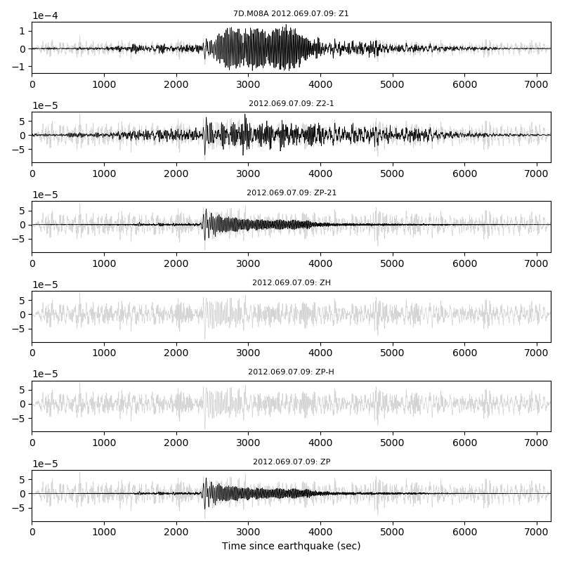
Plot the raw traces
>>> import obstools.atacr.plotting as atplot
>>> figure = atplot.fig_event_raw(evstream, fmin=1./150., fmax=2.)
>>> figure.show()
- correct_data(tfnoise)[source]
Method to apply transfer functions between multiple components (and component combinations) to produce corrected/cleaned vertical components.
- Parameters:
tfnoise (
TFNoise) – Object that contains the noise transfer functions used in the correction
- correct
Container Dictionary for all possible corrections from the transfer functions
- Type:
Examples
Let’s carry through the correction of the vertical component for a single day of noise, say corresponding to the noise recorded on March 04, 2012. In practice, the DayNoise object should correspond to the same day at that of the recorded earthquake to avoid bias in the correction.
>>> from obstools.atacr import DayNoise, TFNoise, EventStream
>>> daynoise = DayNoise('demo')
Uploading demo data - March 04, 2012, station 7D.M08A
>>> daynoise.QC_daily_spectra()
>>> daynoise.average_daily_spectra()
>>> tfnoise_day = TFNoise(daynoise)
>>> tfnoise_day.transfer_func()
>>> evstream = EventStream('demo')
Uploading demo earthquake data - March 09, 2012, station 7D.M08A
>>> evstream.correct_data(tfnoise_day)
Plot the corrected traces
>>> import obstools.atacr.plotting as atplot
>>> figure = atplot.fig_event_corrected(evstream, tfnoise_day.tf_list)
>>> figure.show()
Carry out the same exercise but this time using a StaNoise object
>>> from obstools.atacr import StaNoise, TFNoise, EventStream
>>> stanoise = StaNoise('demo')
Uploading demo data - March 01 to 04, 2012, station 7D.M08A
>>> stanoise.QC_sta_spectra()
>>> stanoise.average_sta_spectra()
>>> tfnoise_sta = TFNoise(stanoise)
>>> tfnoise_sta.transfer_func()
>>> evstream = EventStream('demo')
Uploading demo earthquake data - March 09, 2012, station 7D.M08A
>>> evstream.correct_data(tfnoise_sta)
Plot the corrected traces
>>> import obstools.atacr.plot as plot
>>> plot.fig_event_corrected(evstream, tfnoise_sta.tf_list)
Warning
If the noise window and event window are not identical, they cannot be compared on the same frequency axis and the code will exit. Make sure you are using identical time samples in both the noise and event windows.
- save(filename)[source]
Method to save the object to file using ~Pickle.
- Parameters:
filename (str) – File name
Examples
Following from the example outlined in method
correct_data(), we simply save the final object>>> evstream.save('evstream_demo.pkl')
Check that object has been saved
>>> import glob
>>> glob.glob("./evstream_demo.pkl")
['./evstream_demo.pkl']
Container Classes
Power
- class obstools.atacr.classes.Power(c11=None, c22=None, cZZ=None, cPP=None)[source]
Container for power spectra for each component, with any shape
- c11
Power spectral density for component 1 (any shape)
- Type:
ndarray
- c22
Power spectral density for component 2 (any shape)
- Type:
ndarray
- cZZ
Power spectral density for component Z (any shape)
- Type:
ndarray
- cPP
Power spectral density for component P (any shape)
- Type:
ndarray
Cross
- class obstools.atacr.classes.Cross(c12=None, c1Z=None, c1P=None, c2Z=None, c2P=None, cZP=None)[source]
Container for cross-power spectra for each component pairs, with any shape
- c12
Cross-power spectral density for components 1 and 2 (any shape)
- Type:
ndarray
- c1Z
Cross-power spectral density for components 1 and Z (any shape)
- Type:
ndarray
- c1P
Cross-power spectral density for components 1 and P (any shape)
- Type:
ndarray
- c2Z
Cross-power spectral density for components 2 and Z (any shape)
- Type:
ndarray
- c2P
Cross-power spectral density for components 2 and P (any shape)
- Type:
ndarray
- cZP
Cross-power spectral density for components Z and P (any shape)
- Type:
ndarray
Rotation
- class obstools.atacr.classes.Rotation(cHH=None, cHZ=None, cHP=None, coh=None, ph=None, ad=None, tilt_dir=None, tilt_ang=None, coh_value=None, phase_value=None, admit_value=None, phi=None)[source]
Container for rotated spectra, with any shape
- cHH
Power spectral density for rotated horizontal component H (any shape)
- Type:
ndarray
- cHZ
Cross-power spectral density for components H and Z (any shape)
- Type:
ndarray
- cHP
Cross-power spectral density for components H and P (any shape)
- Type:
ndarray
- coh
Coherence between horizontal-vertical components
- Type:
ndarray
- ph
Phase of cross-power spectrum between horizontal-vertical components
- Type:
ndarray
- ad
Admittance between horizontal-vertical components
- Type:
ndarray
- tilt_dir
Azimuth of the tilt axis
- Type:
float
- tilt_ang
Angle of the tilt axis
- Type:
float
- coh_value
Maximum coherence
- Type:
float
- phase_value
Phase at maximum coherence
- Type:
float
- admit_value
Admittance value at maximum coherence
- Type:
float
- phi
Directions for which the coherence is calculated
- Type:
ndarray
Utility functions
utils contains several functions that are used in the
class methods of ~obstools.atacr.classes.
- obstools.atacr.utils.traceshift(trace, tt)[source]
Function to shift traces in time given travel time
- Parameters:
trace (
Traceobject) – Trace object to updatett (float) – Time shift in seconds
- Returns:
rtrace – Updated trace object
- Return type:
Traceobject
- obstools.atacr.utils.QC_streams(start, end, st)[source]
Function for quality control of traces, which compares the start and end times that were requested, as well as the total n length of the traces.
- Parameters:
start (
UTCDateTimeobject) – Start time of requested streamend (
UTCDateTimeobject) – End time of requested streamst (
Streamobject) – Stream object with all trace data
- Returns:
(pass) (bool) – Whether the QC test has passed
st (
Streamobject) – Updated stream object
- obstools.atacr.utils.update_stats(tr, stla, stlo, stel, cha, evla=None, evlo=None)[source]
Function to include SAC metadata to
Traceobjects- Parameters:
tr (
Traceobject) – Trace object to updatestla (float) – Latitude of station
stlo (float) – Longitude of station
stel (float) – Station elevation (m)
cha (str) – Channel for component
evla (float, optional) – Latitude of event
evlo (float, optional) – Longitute of event
- Returns:
tr – Updated trace object
- Return type:
Traceobject
- obstools.atacr.utils.get_data(datapath, tstart, tend)[source]
Function to grab all available noise data given a path and data time range
- Parameters:
datapath (str) – Path to noise data folder
tstart (
UTCDateTime) – Start time for querytend (
UTCDateTime) – End time for query
- Returns:
tr1, tr2, trZ, trP – Corresponding trace objects for components H1, H2, HZ and HP. Returns empty traces for missing components.
- Return type:
Traceobject
- obstools.atacr.utils.get_event(eventpath, tstart, tend)[source]
Function to grab all available earthquake data given a path and data time range
- Parameters:
eventpath (str) – Path to earthquake data folder
tstart (
UTCDateTime) – Start time for querytend (
UTCDateTime) – End time for query
- Returns:
tr1, tr2, trZ, trP – Corresponding trace objects for components H1, H2, HZ and HP. Returns empty traces for missing components.
- Return type:
Traceobject
- obstools.atacr.utils.calculate_tilt(ft1, ft2, ftZ, ftP, f, goodwins, tiltfreqs, fig_trf=False, savefig=None)[source]
Determines tilt orientation from the maximum coherence between rotated H1 and Z.
- Parameters:
ft1 (
ndarray) – Fourier transform of corresponding H1, H2, HZ and HP componentsft2 (
ndarray) – Fourier transform of corresponding H1, H2, HZ and HP componentsftZ (
ndarray) – Fourier transform of corresponding H1, H2, HZ and HP componentsftP (
ndarray) – Fourier transform of corresponding H1, H2, HZ and HP componentsf (
ndarray) – Frequency axis in Hzgoodwins (list) – List of booleans representing whether a window is good (True) or not (False). This attribute is returned from the method
QC_daily_spectra()tiltfreqs (list) – Two floats representing the frequency band at which the mean coherence, phase and admittance are calculated to determine the tile orientation
- Returns:
cHH, cHZ, cHP (
ndarray) – Arrays of power and cross-spectral density functions of components HH (rotated H1 in direction of maximum tilt), HZ, and HPcoh (
ndarray) – Mean coherence value between rotated H and Z components, as a function of azimuth CW from H1ph (
ndarray) – Mean phase value between rotated H and Z components, as a function of azimuth CW from H1ad (
ndarray) – Mean admittance value between rotated H and Z components, as a function of azimuth CW from H1phi (
ndarray) – Array of azimuths CW from H1 consideredtilt_dir (float) – Tilt direction (azimuth CW from H1) at maximum coherence between rotated H1 and Z
tilt_ang (float) – Tilt angle (down from HZ/3) at maximum coherence between rotated H1 and Z
coh_value (float) – Mean coherence value at tilt direction
phase_value (float) – Mean phase value at tilt direction
admit_value (float) – Mean admittance value at tilt direction
- obstools.atacr.utils.smooth(data, nd, axis=0)[source]
Function to smooth power spectral density functions from the convolution of a boxcar function with the PSD
- Parameters:
data (
ndarray) – Real-valued array to smooth (PSD)nd (int) – Number of samples over which to smooth
axis (int, optional) – axis over which to perform the smoothing
- Returns:
filt – Filtered data
- Return type:
ndarray, optional
- obstools.atacr.utils.admittance(Gxy, Gxx)[source]
Calculates admittance between two components
- Parameters:
Gxy (
ndarray) – Cross spectral density function of x and yGxx (
ndarray) – Power spectral density function of x
- Returns:
Admittance between x and y
- Return type:
ndarray, optional
- obstools.atacr.utils.coherence(Gxy, Gxx, Gyy)[source]
Calculates coherence between two components
- Parameters:
Gxy (
ndarray) – Cross spectral density function of x and yGxx (
ndarray) – Power spectral density function of xGyy (
ndarray) – Power spectral density function of y
- Returns:
Coherence between x and y
- Return type:
ndarray, optional
- obstools.atacr.utils.phase(Gxy)[source]
Calculates phase angle between real and imaginary components
- Parameters:
Gxy (
ndarray) – Cross spectral density function of x and y- Returns:
Phase angle between x and y
- Return type:
ndarray, optional
- obstools.atacr.utils.rotate_dir(x, y, theta)[source]
Rotates (x, y) data clockwise by an angle theta. Returns the rotated component y.
- Parameters:
x (
ndarray) – Array of values along the x coordinatey (
ndarray) – Array of values along the y coordinatetheta (
ndarray) – Angle in degrees
- Returns:
y_rotated – Rotated array of component y
- Return type:
ndarray
Plotting functions
plot contains several functions for plotting the results
of the analysis at various final and intermediate steps.
- obstools.atacr.plotting.fig_QC(f, power, gooddays, ncomp, key='')[source]
Function to plot the Quality-Control step of the analysis. This function is used in both the atacr_daily_spectra or atacr_clean_spectra scripts.
- Parameters:
f (
ndarray) – Frequency axis (in Hz)power (
Power) – Container for the Power spectragooddays (List) – List of booleans representing whether a window is good (True) or not (False)
ncomp (int) – Number of components used in analysis (can be 2, 3 or 4)
key (str) – String corresponding to the station key under analysis
- obstools.atacr.plotting.fig_average(f, power, bad, gooddays, ncomp, key='')[source]
Function to plot the averaged spectra (those qualified as ‘good’ in the QC step). This function is used in both the atacr_daily_spectra or atacr_clean_spectra scripts.
- Parameters:
f (
ndarray) – Frequency axis (in Hz)power (
Power) – Container for the Power spectrabad (
Power) – Container for the bad Power spectragooddays (List) – List of booleans representing whether a window is good (True) or not (False)
ncomp (int) – Number of components used in analysis (can be 2, 3 or 4)
key (str) – String corresponding to the station key under analysis
- obstools.atacr.plotting.fig_av_cross(f, field, gooddays, ftype, ncomp, key='', save=False, fname='', form='png', **kwargs)[source]
Function to plot the averaged cross-spectra (those qualified as ‘good’ in the QC step). This function is used in the atacr_daily_spectra script.
- Parameters:
f (
ndarray) – Frequency axis (in Hz)field (
Rotation) – Container for the Power spectragooddays (List) – List of booleans representing whether a window is good (True) or not (False)
ftype (str) – Type of plot to be displayed. If ftype is Admittance, plot is loglog. Otherwise semilogx
key (str) – String corresponding to the station key under analysis
**kwargs (None) – Keyword arguments to modify plot
- obstools.atacr.plotting.fig_tilt_date(gooddays, coh, ph, ad, phi, tilt_dir, tilt_ang, date)[source]
Function to plot the coherence, phase and admittance between the rotated H and Z components, used to characterize the tilt orientation, for a range of dates.
- Parameters:
gooddays (
ndarray) – Array of gooddays to use in showing the resultscoh (
ndarray) – Coherence between rotated H and Z componentsph (
ndarray) – Phase between rotated H and Z componentsad (
ndarray) – Admittance between rotated H and Z componentsphi (
ndarray) – Directions considered in maximizing coherence between H and Ztilt_dir (list) – List of tilt directions determined for each date
tilt_ang (list) – List of tilt angles determined for each date
date (list) – List of datetime dates for plotting as function of time
- obstools.atacr.plotting.fig_tilt_day(coh_phi, ph_phi, ad_phi, phi, coh_spec, ph_spec, ad_spec, f, f_tilt, tilt_dir, tilt_ang)[source]
Function to plot the coherence, phase and admittance between the rotated H and Z components, used to characterize the tilt orientation, for a single day. The figure also includes the transfer function components.
- Parameters:
coh_phi (
ndarray) – Coherence between rotated H and Z components as function of the direction phiph_phi (
ndarray) – Phase between rotated H and Z components as function of the direction phiad_phi (
ndarray) – Admittance between rotated H and Z components as function of the direction phiphi (
ndarray) – Directions phi considered in maximizing coherence between H and Zcoh_spec (
ndarray) – Coherence spectrum between rotated H and Z components at the direction where coherence is maximum, as function of frequencyph_spec (
ndarray) – Phase spectrum between rotated H and Z components at the direction where coherence is maximum, as function of frequencyad_spec (
ndarray) – Admittance spectrum between rotated H and Z components at the direction where coherence is maximum, as function of frequencyf (
ndarray) – Frequency axisf_tilt (
ndarray) – Frequencies used in tilt calculationtilt_dir (float) – Tilt direction
tilt_ang (float) – Tilt angle
- obstools.atacr.plotting.fig_TF(f, day_trfs, day_list, sta_trfs={}, sta_list={}, skey='')[source]
Function to plot the transfer functions available.
- Parameters:
f (
ndarray) – Frequency axis (in Hz)day_trfs (Dict) – Dictionary containing the transfer functions for the daily averages
day_list (Dict) – Dictionary containing the list of daily transfer functions
sta_trfs (Dict) – Dictionary containing the transfer functions for the station averages
sta_list (Dict) – Dictionary containing the list of average transfer functions
skey (str) – String corresponding to the station key under analysis
- obstools.atacr.plotting.fig_comply(f, day_comps, day_list, sta_comps, sta_list, skey=None, elev=-1000.0, f_0=None, f_1=None, log=False)[source]
Function to plot the transfer functions available.
- Parameters:
f (
ndarray) – Frequency axis (in Hz)day_comps (Dict) – Dictionary containing the compliance functions for the daily averages
day_list (Dict) – Dictionary containing the list of daily transfer functions
sta_comps (Dict) – Dictionary containing the compliance functions for the station averages
sta_list (Dict) – Dictionary containing the list of average transfer functions
skey (str) – String corresponding to the station key under analysis
elev (float) – Station elevation in meters (OBS stations have negative elevations)
f_0 (float) – Lowest frequency to consider in plot (Hz)
f_1 (float) – Highest frequency to consider in plot (Hz)
log (boolean) – Show a logarithmic frequency axis for compliance
- obstools.atacr.plotting.fig_event_raw(evstream, fmin=0.006666666666666667, fmax=2.0)[source]
Function to plot the raw (although bandpassed) seismograms.
- Parameters:
evstream (
EventStream) – Container for the event stream datafmin (float) – Low frequency corner (in Hz)
fmax (float) – High frequency corner (in Hz)
- obstools.atacr.plotting.fig_event_corrected(evstream, TF_list, fmin=0.006666666666666667, fmax=2.0)[source]
Function to plot the corrected vertical component seismograms.
- Parameters:
evstream (
EventStream) – Container for the event stream dataTf_list (list) – List of Dictionary elements of transfer functions used for plotting the corrected vertical component.
Scripts
There are several Python scripts that accompany ~obstools.atacr. These can be used
in bash scripts to automate data processing. These include scripts to download noise and
event data, and perform tilt and compliance noise removal using either the default
program values or by refining parameters. All of them use a station database provided as a
StDb dictionary. These scripts are:
atacr_download_data
atacr_download_event
atacr_daily_spectra
atacr_clean_spectra
atacr_transfer_functions
atacr_correct_event
atacr_download_data
Description
Downloads up to four-component (1, 2, Z and P), day-long seismograms
to use in noise corrections of vertical
component data. Station selection is specified by a network and
station code. The database is provided as a StDb dictionary.
Usage
$ atacr_download_data -h

###########################################################################
#      _                     _                 _        _       _         #
#   __| | _____      ___ __ | | ___   __ _  __| |    __| | __ _| |_ __ _  #
#  / _` |/ _ \ \ /\ / / '_ \| |/ _ \ / _` |/ _` |   / _` |/ _` | __/ _` | #
# | (_| | (_) \ V  V /| | | | | (_) | (_| | (_| |  | (_| | (_| | || (_| | #
#  \__,_|\___/ \_/\_/ |_| |_|_|\___/ \__,_|\__,_|___\__,_|\__,_|\__\__,_| #
#                                              |_____|                    #
#                                                                         #
###########################################################################

usage: atacr_download_data [options] <indb>

Script used to download and pre-process up to four-component (H1, H2, Z and P), day-long
seismograms to use in noise corrections of vertical component of OBS data. Data are requested
from the internet using the client services framework for a given date range. The stations
are processed one by one and the data are stored to disk.

positional arguments:
  indb                  Station Database to process from. Available formats are:
                        StDb (.pkl or .csv) or stationXML (.xml)

options:
  -h, --help            show this help message and exit
  --keys STKEYS         Specify a comma-separated list of station keys for which to perform
                        the analysis. These must be contained within the station database.
                        Partial keys will be used to match against those in the dictionary.
                        For instance, providing IU will match with all stations in the IU
                        network. [Default processes all stations in the database]
  -O, --overwrite       Force the overwriting of pre-existing data. [Default False]
  -Z ZCOMP, --zcomp ZCOMP
                        Specify the Vertical Component Channel Identifier. [Default Z].

Server Settings:
  Settings associated with FDSN datacenters for archived data.

  --server SERVER       Base URL of FDSN web service compatible server (e.g.
                        “http://service.iris.edu”) or key string for recognized server (one
                        of 'AUSPASS', 'BGR', 'EARTHSCOPE', 'EIDA', 'EMSC', 'ETH', 'GEOFON',
                        'GEONET', 'GFZ', 'ICGC', 'IESDMC', 'INGV', 'IPGP', 'IRIS', 'IRISPH5',
                        'ISC', 'KNMI', 'KOERI', 'LMU', 'NCEDC', 'NIEP', 'NOA', 'NRCAN',
                        'ODC', 'ORFEUS', 'RASPISHAKE', 'RESIF', 'RESIFPH5', 'SCEDC',
                        'TEXNET', 'UIB-NORSAR', 'USGS', 'USP'). [Default 'IRIS']
  --user-auth USERAUTH  Authentification Username and Password for the waveform server
                        (--user-auth='username:authpassword') to access and download
                        restricted data. [Default no user and password]
  --eida-token TOKENFILE
                        Token for EIDA authentication mechanism, see http://geofon.gfz-
                        potsdam.de/waveform/archive/auth/index.php. If a token is provided,
                        argument --user-auth will be ignored. This mechanism is only
                        available on select EIDA nodes. The token can be provided in form of
                        the PGP message as a string, or the filename of a local file with the
                        PGP message in it. [Default None]

Local Data Settings:
  Settings associated with a SeisComP database for locally archived data.

  --SDS-path LOCALDATA  Specify absolute path to a SeisComP Data Structure (SDS) archive containing
                        day-long SAC or MSEED files(e.g., --SDS-path=/Home/username/Data/SDS). See
                        https://www.seiscomp.de/seiscomp3/doc/applications/slarchive/SDS.html for
                        details on the SDS format. If this option is used, it takes precedence over
                        the --server settings.
  --dtype DTYPE         Specify the data archive file type, either SAC or MSEED. Note the
                        default behaviour is to search for SAC files. Local archive files
                        must have extensions of '.SAC' or '.MSEED'. These are case dependent,
                        so specify the correct case here.

Frequency Settings:
  Miscellaneous frequency settings

  --sampling-rate NEW_SAMPLING_RATE
                        Specify new sampling rate (float, in Hz). [Default 5.]
  --units UNITS         Choose the output seismogram units. Options are: 'DISP', 'VEL',
                        'ACC'. [Default 'DISP']
  --pre-filt PRE_FILT   Specify four comma-separated corner frequencies (float, in Hz) for
                        deconvolution pre-filter. [Default 0.001,0.005,45.,50.]

Time Search Settings:
  Time settings associated with searching for day-long seismograms

  --start STARTT        Specify a UTCDateTime compatible string representing the start day
                        for the data search. This will override any station start times.
                        [Default start date for each station in database]
  --end ENDT            Specify a UTCDateTime compatible string representing the start time
                        for the event search. This will override any station end times
                        [Default end date for each station in database]
atacr_daily_spectra
Description
Extracts two-hour-long windows from the day-long data, calculates
power-spectral densities and flags windows for outlier from the PSD properties.
Station selection is specified by a network and station code. The database
is provided as a StDb dictionary.
Usage
$ atacr_daily_spectra -h

#################################################################
#      _       _ _                               _              #
#   __| | __ _(_) |_   _     ___ _ __   ___  ___| |_ _ __ __ _  #
#  / _` |/ _` | | | | | |   / __| '_ \ / _ \/ __| __| '__/ _` | #
# | (_| | (_| | | | |_| |   \__ \ |_) |  __/ (__| |_| | | (_| | #
#  \__,_|\__,_|_|_|\__, |___|___/ .__/ \___|\___|\__|_|  \__,_| #
#                  |___/_____|  |_|                             #
#                                                               #
#################################################################

usage: atacr_daily_spectra [options] <indb>

Script used to extract shorter windows from the day-long seismograms,
calculate the power-spectral properties, flag windows for outlier PSDs and
calculate daily averages of the corresponding Fourier transforms. The stations
are processed one by one and the data are stored to disk. The program will
look for data saved in the previous steps and use all available components.

positional arguments:
  indb               Station Database to process from. Available formats are:
                     StDb (.pkl or .csv) or stationXML (.xml)

optional arguments:
  -h, --help         show this help message and exit
  --keys STKEYS      Specify a comma separated list of station keys for which
                     to perform the analysis. These must be contained within
                     the station database. Partial keys will be used to match
                     against those in the dictionary. For instance, providing
                     IU will match with all stations in the IU network.
                     [Default processes all stations in the database]
  -O, --overwrite    Force the overwriting of pre-existing data. [Default
                     False]

Time Search Settings:
  Time settings associated with searching for day-long seismograms

  --start STARTT     Specify a UTCDateTime compatible string representing the
                     start day for the data search. This will override any
                     station start times. [Default start date of each station
                     in database]
  --end ENDT         Specify a UTCDateTime compatible string representing the
                     start time for the data search. This will override any
                     station end times. [Default end date of each station n
                     database]

Parameter Settings:
  Miscellaneous default values and settings

  --window WINDOW    Specify window length in seconds. Default value is highly
                     recommended. Program may not be stable for large
                     deviations from default value. [Default 7200. (or 2
                     hours)]
  --overlap OVERLAP  Specify fraction of overlap between windows. [Default 0.3
                     (or 30 percent)]
  --minwin MINWIN    Specify minimum number of 'good' windows in any given day
                     to continue with analysis. [Default 10]
  --flag-freqs PD    Specify comma-separated frequency limits (float, in Hz) over which to
                     calculate spectral features used in flagging the bad windows. [Default
                     0.004,2.0]
  --tilt-freqs TF    Specify comma-separated frequency limits (float, in Hz) over which to
                     calculate tilt. [Default 0.005,0.035]
  --tolerance TOL    Specify parameter for tolerance threshold. If spectrum >
                     std*tol, window is flagged as bad. [Default 2.0]
  --alpha ALPHA      Specify confidence level for f-test, for iterative
                     flagging of windows. [Default 0.05, or 95 percent
                     confidence]
  --raw              Raw spectra will be used in calculating spectral features
                     for flagging. [Default uses smoothed spectra]
  --no-rotation      Do not rotate horizontal components to tilt direction.
                     [Default calculates rotation]

Figure Settings:
  Flags for plotting figures

  --figQC            Plot Quality-Control figure. [Default does not plot
                     figure]
  --debug            Plot intermediate steps for debugging. [Default does not
                     plot figure]
  --figAverage       Plot daily average figure. [Default does not plot figure]
  --figCoh           Plot Coherence and Phase figure. [Default does not plot
                     figure]
  --save-fig         Set this option if you wish to save the figure(s).
                     [Default does not save figure]
  --format FORM      Specify format of figure. Can be any one of the
                     validmatplotlib formats: 'png', 'jpg', 'eps', 'pdf'.
                     [Default 'png']
atacr_clean_spectra
Description
Extracts daily spectra calculated from atacr_daily_spectra and
flags days for which the daily averages are outliers from the PSD properties.
Further averages the spectra over the whole period specified by --start
and --end. Station selection is specified by a network and station code.
The database is provided as a StDb dictionary.
Usage
$ atacr_clean_spectra -h

###################################################################
#       _                                          _              #
#   ___| | ___  __ _ _ __      ___ _ __   ___  ___| |_ _ __ __ _  #
#  / __| |/ _ \/ _` | '_ \    / __| '_ \ / _ \/ __| __| '__/ _` | #
# | (__| |  __/ (_| | | | |   \__ \ |_) |  __/ (__| |_| | | (_| | #
#  \___|_|\___|\__,_|_| |_|___|___/ .__/ \___|\___|\__|_|  \__,_| #
#                        |_____|  |_|                             #
#                                                                 #
###################################################################

usage: atacr_clean_spectra [options] <indb>

Script used to extract daily spectra calculated from `obs_daily_spectra.py`
and flag days for outlier PSDs and calculate spectral averages of the
corresponding Fourier transforms over the entire time period specified. The
stations are processed one by one and the data are stored to disk.

positional arguments:
  indb             Station Database to process from. Available formats are:
                   StDb (.pkl or .csv) or stationXML (.xml)

optional arguments:
  -h, --help       show this help message and exit
  --keys STKEYS    Specify a comma separated list of station keys for which to
                   perform the analysis. These must be contained within the
                   station database. Partial keys will be used to match
                   against those in the dictionary. For instance, providing IU
                   will match with all stations in the IU network. [Default
                   processes all stations in the database]
  -O, --overwrite  Force the overwriting of pre-existing data. [Default False]

Time Search Settings:
  Time settings associated with searching for day-long seismograms

  --start STARTT   Specify a UTCDateTime compatible string representing the
                   start day for the data search. This will override any
                   station start times. [Default start date of each station in
                   database]
  --end ENDT       Specify a UTCDateTime compatible string representing the
                   start time for the data search. This will override any
                   station end times. [Default end date of each station in
                   database]

Parameter Settings:
  Miscellaneous default values and settings

  --flag-freqs PD  Specify comma-separated frequency limits (float, in Hz) over which to
                   calculate spectral features used in flagging the days/windows. [Default
                   0.004,2.0]
  --tolerance TOL  Specify parameter for tolerance threshold. If spectrum >
                   std*tol, window is flagged as bad. [Default 1.5]
  --alpha ALPHA    Confidence level for f-test, for iterative flagging of
                   windows. [Default 0.05, or 95 percent confidence]

Figure Settings:
  Flags for plotting figures

  --figQC          Plot Quality-Control figure. [Default does not plot figure]
  --debug          Plot intermediate steps for debugging. [Default does not
                   plot figure]
  --figAverage     Plot daily average figure. [Default does not plot figure]
  --figTilt        Plot coherence, phase and tilt direction figure. [Default does not plot
                   figure]
  --figCross       Plot cross-spectra figure. [Default does not plot figure]
  --save-fig       Set this option if you wish to save the figure(s). [Default
                   does not save figure]
  --format FORM    Specify format of figure. Can be any one of the
                   validmatplotlib formats: 'png', 'jpg', 'eps', 'pdf'.
                   [Default 'png']
atacr_transfer functions
Description
Calculates transfer functions using the noise windows flagged as good, for either
a single day (from atacr_daily_spectra) or for those averaged over several days
(from atacr_clean_spectra), if available. The transfer functions are stored to disk.
Station selection is specified by a network and station code. The database is
provided as a StDb dictionary.
Usage
$ atacr_transfer_functions -h

#######################################################################################
#  _                        __             __                  _   _                  #
# | |_ _ __ __ _ _ __  ___ / _| ___ _ __  / _|_   _ _ __   ___| |_(_) ___  _ __  ___  #
# | __| '__/ _` | '_ \/ __| |_ / _ \ '__|| |_| | | | '_ \ / __| __| |/ _ \| '_ \/ __| #
# | |_| | | (_| | | | \__ \  _|  __/ |   |  _| |_| | | | | (__| |_| | (_) | | | \__ \ #
#  \__|_|  \__,_|_| |_|___/_|  \___|_|___|_|  \__,_|_| |_|\___|\__|_|\___/|_| |_|___/ #
#                                   |_____|                                           #
#                                                                                     #
#######################################################################################

usage: atacr_transfer_functions [options] <indb>

Script used to calculate transfer functions between various components, to be
used in cleaning vertical component of OBS data. The noise data can be those
obtained from the daily spectra (i.e., from `atacr_daily_spectra`) or those
obtained from the averaged noise spectra (i.e., from `atacr_clean_spectra`).
Flags are available to specify the source of data to use as well as the time
range over which to calculate the transfer functions. The stations are
processed one by one and the data are stored to disk.

positional arguments:
  indb             Station Database to process from. Available formats are:
                   StDb (.pkl or .csv) or stationXML (.xml)

optional arguments:
  -h, --help       show this help message and exit
  --keys STKEYS    Specify a comma separated list of station keys for which to
                   perform the analysis. These must be contained within the
                   station database. Partial keys will be used to match
                   against those in the dictionary. For instance, providing IU
                   will match with all stations in the IU network. [Default
                   processes all stations in the database]
  -O, --overwrite  Force the overwriting of pre-existing data. [Default False]

Time Search Settings:
  Time settings associated with searching for day-long seismograms

  --start STARTT   Specify a UTCDateTime compatible string representing the
                   start day for the data search. This will override any
                   station start times. [Default start date of each station in
                   database]
  --end ENDT       Specify a UTCDateTime compatible string representing the
                   start time for the data search. This will override any
                   station end times. [Default end date of each station in
                   database]

Parameter Settings:
  Miscellaneous default values and settings

  --skip-daily     Skip daily spectral averages in construction of transfer
                   functions. [Default False]
  --skip-clean     Skip cleaned spectral averages in construction of transfer
                   functions. Defaults to True if data cannot be found in
                   default directory. [Default False]

Figure Settings:
  Flags for plotting figures

  --figTF          Plot transfer function figure. [Default does not plot
                   figure]
  --save-fig       Set this option if you wish to save the figure(s). [Default
                   does not save figure]
  --format FORM    Specify format of figure. Can be any one of the
                   validmatplotlib formats: 'png', 'jpg', 'eps', 'pdf'.
                   [Default 'png']
atacr_download_event
Description
Downloads up to four-component (1,2,Z,H), two-hour-long seismograms
for individual seismic events to use in noise corrections of vertical
component data. Station selection is specified by a network and
station code. The database is provided as a StDb dictionary.
Usage
$ atacr_download_event -h

###############################################################################
#      _                     _                 _                         _    #
#   __| | _____      ___ __ | | ___   __ _  __| |    _____   _____ _ __ | |_  #
#  / _` |/ _ \ \ /\ / / '_ \| |/ _ \ / _` |/ _` |   / _ \ \ / / _ \ '_ \| __| #
# | (_| | (_) \ V  V /| | | | | (_) | (_| | (_| |  |  __/\ V /  __/ | | | |_  #
#  \__,_|\___/ \_/\_/ |_| |_|_|\___/ \__,_|\__,_|___\___| \_/ \___|_| |_|\__| #
#                                              |_____|                        #
#                                                                             #
###############################################################################

usage: atacr_download_event [options] <indb>

Script used to download and pre-process four-component (H1, H2, Z and P), two-hour-long
seismograms for individual events on which to apply the de-noising algorithms. Data are
requested from the internet using the client services framework for a given date range. The
stations are processed one by one and the data are stored to disk.

positional arguments:
  indb                  Station Database to process from. Available formats are:
                        StDb (.pkl or .csv) or stationXML (.xml)

options:
  -h, --help            show this help message and exit
  --keys STKEYS         Specify a comma separated list of station keys for which to perform
                        the analysis. These must be contained within the station database.
                        Partial keys will be used to match against those in the dictionary.
                        For instance, providing IU will match with all stations in the IU
                        network [Default processes all stations in the database]
  -O, --overwrite       Force the overwriting of pre-existing data. [Default False]
  --zcomp ZCOMP         Specify the Vertical Component Channel Identifier. [Default Z].

Server Settings:
  Settings associated with FDSN datacenters for archived data.

  --server SERVER       Base URL of FDSN web service compatible server (e.g.
                        “http://service.iris.edu”) or key string for recognized server (one
                        of 'AUSPASS', 'BGR', 'EARTHSCOPE', 'EIDA', 'EMSC', 'ETH', 'GEOFON',
                        'GEONET', 'GFZ', 'ICGC', 'IESDMC', 'INGV', 'IPGP', 'IRIS', 'IRISPH5',
                        'ISC', 'KNMI', 'KOERI', 'LMU', 'NCEDC', 'NIEP', 'NOA', 'NRCAN',
                        'ODC', 'ORFEUS', 'RASPISHAKE', 'RESIF', 'RESIFPH5', 'SCEDC',
                        'TEXNET', 'UIB-NORSAR', 'USGS', 'USP'). [Default 'IRIS']
  --user-auth USERAUTH  Authentification Username and Password for the waveform server
                        (--user-auth='username:authpassword') to access and download
                        restricted data. [Default no user and password]
  --eida-token TOKENFILE
                        Token for EIDA authentication mechanism, see http://geofon.gfz-
                        potsdam.de/waveform/archive/auth/index.php. If a token is provided,
                        argument --user-auth will be ignored. This mechanism is only
                        available on select EIDA nodes. The token can be provided in form of
                        the PGP message as a string, or the filename of a local file with the
                        PGP message in it. [Default None]

Local Data Settings:
  Settings associated with a SeisComP database for locally archived data.

  --SDS-path LOCALDATA  Specify absolute path to a SeisComP Data Structure (SDS) archive containing
                        day-long SAC or MSEED files(e.g., --SDS-path=/Home/username/Data/SDS). See
                        https://www.seiscomp.de/seiscomp3/doc/applications/slarchive/SDS.html for
                        details on the SDS format. If this option is used, it takes precedence over
                        the --server settings.
  --dtype DTYPE         Specify the data archive file type, either SAC or MSEED. Note the
                        default behaviour is to search for SAC files. Local archive files
                        must have extensions of '.SAC' or '.MSEED'. These are case dependent,
                        so specify the correct case here.

Frequency Settings:
  Miscellaneous frequency settings

  --sampling-rate NEW_SAMPLING_RATE
                        Specify new sampling rate (float, in Hz). [Default 5.]
  --units UNITS         Choose the output seismogram units. Options are: 'DISP', 'VEL',
                        'ACC'. [Default 'DISP']
  --pre-filt PRE_FILT   Specify four comma-separated corner frequencies (float, in Hz) for
                        deconvolution pre-filter. [Default 0.001,0.005,45.,50.]
  --window WINDOW       Specify window length in seconds. Default value is highly
                        recommended. Program may not be stable for large deviations from
                        default value. [Default 7200. (or 2 hours)]

Event Settings:
  Settings associated with refining the events to include in matching station pairs

  --start STARTT        Specify a UTCDateTime compatible string representing the start time
                        for the event search. This will override any station start times.
                        [Default start date of each station in database]
  --end ENDT            Specify a UTCDateTime compatible string representing the start time
                        for the event search. This will override any station end times
                        [Default end date of each station in database]
  --reverse-order, -R   Reverse order of events. Default behaviour starts at oldest event and
                        works towards most recent. Specify reverse order and instead the
                        program will start with the most recent events and work towards older
  --min-mag MINMAG      Specify the minimum magnitude of event for which to search. [Default
                        5.5]
  --max-mag MAXMAG      Specify the maximum magnitude of event for which to search. [Default
                        None, i.e. no limit]

Geometry Settings:
  Settings associatd with the event-station geometries

  --min-dist MINDIST    Specify the minimum great circle distance (degrees) between the
                        station and event. [Default 30]
  --max-dist MAXDIST    Specify the maximum great circle distance (degrees) between the
                        station and event. [Default 120]
atacr_correct_event
Description
Loads the transfer functions previously calculated and performs the noise corrections, for either
a single day (from atacr_daily_spectra) or for those averaged over several days
(from atacr_clean_spectra), if available. The database is provided as a
StDb dictionary.
Usage
$ atacr_correct_event -h

##################################################################
#                               _                           _    #
#   ___ ___  _ __ _ __ ___  ___| |_     _____   _____ _ __ | |_  #
#  / __/ _ \| '__| '__/ _ \/ __| __|   / _ \ \ / / _ \ '_ \| __| #
# | (_| (_) | |  | | |  __/ (__| |_   |  __/\ V /  __/ | | | |_  #
#  \___\___/|_|  |_|  \___|\___|\__|___\___| \_/ \___|_| |_|\__| #
#                                 |_____|                        #
#                                                                #
##################################################################

usage: atacr_correct_event [options] <indb>

Script used to extract transfer functions between various components, and use
them to clean vertical component of OBS data for selected events. The noise
data can be those obtained from the daily spectra (i.e., from
`atacr_daily_spectra`) or those obtained from the averaged noise spectra
(i.e., from `atacr_clean_spectra`). Flags are available to specify the source
of data to use as well as the time range for given events. The stations are
processed one by one and the data are stored to disk in a new 'CORRECTED'
folder.

positional arguments:
  indb             Station Database to process from. Available formats are:
                   StDb (.pkl or .csv) or stationXML (.xml)

optional arguments:
  -h, --help       show this help message and exit
  --keys STKEYS    Specify a comma separated list of station keys for which to
                   perform the analysis. These must be contained within the
                   station database. Partial keys will be used to match
                   against those in the dictionary. For instance, providing IU
                   will match with all stations in the IU network. [Default
                   processes all stations in the database]
  -O, --overwrite  Force the overwriting of pre-existing data. [Default False]

Time Search Settings:
  Time settings associated with searching for specific event-related
  seismograms

  --start STARTT   Specify a UTCDateTime compatible string representing the
                   start day for the event search. This will override any
                   station start times. [Default start date of each station in
                   database]
  --end ENDT       Specify a UTCDateTime compatible string representing the
                   start time for the event search. This will override any
                   station end times. [Default end date of each station in
                   database]

Parameter Settings:
  Miscellaneous default values and settings

  --skip-daily     Skip daily spectral averages in application of transfer
                   functions. [Default False]
  --skip-clean     Skip cleaned spectral averages in application of transfer
                   functions. [Default False]
  --fmin FMIN      Low frequency corner (in Hz) for plotting the raw (un-
                   corrected) seismograms. Filter is a 2nd order, zero phase
                   butterworth filter. [Default 1./150.]
  --fmax FMAX      High frequency corner (in Hz) for plotting the raw (un-
                   corrected) seismograms. Filter is a 2nd order, zero phase
                   butterworth filter. [Default 1./10.]

Figure Settings:
  Flags for plotting figures

  --figRaw         Plot raw seismogram figure. [Default does not plot figure]
  --figClean       Plot cleaned vertical seismogram figure. [Default does not
                   plot figure]
  --save-fig       Set this option if you wish to save the figure(s). [Default
                   does not save figure]
  --format FORM    Specify format of figure. Can be any one of the
                   validmatplotlib formats: 'png', 'jpg', 'eps', 'pdf'.
                   [Default 'png']
Tutorial
Note
Here we roughly follow the steps highlighted in the Matlab tutorial for this code and reproduce the various figures. The examples provided below are for one month of data (March 2012) recorded at station M08A of the Cascadia Initiative Experiment. Corrections are applied to a magnitude 6.6 earthquake that occurred near Vanuatu on March 9, 2012.
0. Creating the StDb Database
All the scripts provided require a StDb database containing station
information and metadata. Let’s first create this database for station
M08A and send the prompt to a logfile
$ query_fdsn_stdb -N 7D -S M08A M08A > logfile
To check the station info for M08A, use the program ls_stdb:
$ ls_stdb M08A.pkl
 Listing Station Pickle: M08A.pkl
 7D.M08A
 --------------------------------------------------------------------------
 1) 7D.M08A
      Station: 7D M08A
       Alternate Networks: None
       Channel: BH ;  Location: --
       Lon, Lat, Elev:  44.11870, -124.89530,  -0.126
       StartTime: 2011-10-20 00:00:00
       EndTime:   2012-07-18 23:59:59
       Status:    open
       Polarity: 1
       Azimuth Correction: 0.000000
1. Download noise data
We wish to download one month of data for the station M08A for March 2012.
The program will search for and download all available (1,2,Z,H) data.
Default frequency settings for data pre-processing match those of
the Matlab ATaCR software.
Since the file M08A.pkl contains only one station, it is not necessary to specify a
key. This option would be useful if the database contained several stations
and we were only interested in downloading data for M08A. In this case, we would
specify --keys=M08A or --keys=7D.M08A.
The only required options at this point are the --start and --end options
to specify the dates for which data will be downloaded.
If you change your mind about the pre-processing options, you can always re-run the
following line with the option -O, which will overwrite the data saved to disk.
To download all available data, simply type in a terminal:
$ atacr_download_data --start=2012-03-01 --end=2012-04-01 M08A.pkl
An example log printed on the terminal will look like:
###########################################################################
#      _                     _                 _        _       _         #
#   __| | _____      ___ __ | | ___   __ _  __| |    __| | __ _| |_ __ _  #
#  / _` |/ _ \ \ /\ / / '_ \| |/ _ \ / _` |/ _` |   / _` |/ _` | __/ _` | #
# | (_| | (_) \ V  V /| | | | | (_) | (_| | (_| |  | (_| | (_| | || (_| | #
#  \__,_|\___/ \_/\_/ |_| |_|_|\___/ \__,_|\__,_|___\__,_|\__,_|\__\__,_| #
#                                              |_____|                    #
#                                                                         #
###########################################################################


Path to DATA/7D.M08A doesn't exist - creating it

|===============================================|
|===============================================|
|                       M08A                    |
|===============================================|
|===============================================|
|  Station: 7D.M08A                             |
|      Channel: BH; Locations: --               |
|      Lon: -124.90; Lat:  44.12                |
|      Start time: 2011-10-20                   |
|      End time:   2012-07-18                   |
|-----------------------------------------------|
| Searching day-long files:                     |
|   Start: 2012-03-01                           |
|   End:   2012-04-01                           |

************************************************************
* Downloading day-long data for key 7D.M08A and day 2012.061
*
*   2012.061.*.SAC
*   -> Downloading BH1 data...
*      ...done
*   -> Downloading BH2 data...
*      ...done
*   -> Downloading BHZ data...
*      ...done
*   -> Downloading ?DH data...
*      ...done
* Start times are not all close to true start:
*   BH1 2012-03-01T00:00:00.017800Z 2012-03-01T23:59:58.017800Z
*   BH2 2012-03-01T00:00:00.017800Z 2012-03-01T23:59:58.017800Z
*   BHZ 2012-03-01T00:00:00.017800Z 2012-03-01T23:59:58.017800Z
*   BDH 2012-03-01T00:00:00.017800Z 2012-03-01T23:59:58.017800Z
*   True start: 2012-03-01T00:00:00.000000Z
* -> Shifting traces to true start
*   -> Removing responses - Seismic data
 WARNING: FIR normalized: sum[coef]=9.767192E-01;
 WARNING: FIR normalized: sum[coef]=9.767192E-01;
 WARNING: FIR normalized: sum[coef]=9.767192E-01;
*   -> Removing responses - Pressure data
 WARNING: FIR normalized: sum[coef]=9.767192E-01;

************************************************************
* Downloading day-long data for key 7D.M08A and day 2012.062
*
*   2012.062.*.SAC
*   -> Downloading BH1 data...
*      ...done
*   -> Downloading BH2 data...

...
And so on until all day-long files have been downloaded. You will
notice that a folder called DATA/7D.M08A/ has been created.
This is where all day-long files will be stored on disk.
2. QC for daily spectral averages
For this step, there are several Parameter Settings that can be tuned. Once again, the default values are the ones used to reproduce the results of the Matlab ATaCR software. The Time Search Settings can be used to look at a subset of the available day-long data files. Here these options can be ignored since we wish to look at all the availble data that we just downloaded. We can therefore type in a terminal:
$ atacr_daily_spectra M08A.pkl

#################################################################
#      _       _ _                               _              #
#   __| | __ _(_) |_   _     ___ _ __   ___  ___| |_ _ __ __ _  #
#  / _` |/ _` | | | | | |   / __| '_ \ / _ \/ __| __| '__/ _` | #
# | (_| | (_| | | | |_| |   \__ \ |_) |  __/ (__| |_| | | (_| | #
#  \__,_|\__,_|_|_|\__, |___|___/ .__/ \___|\___|\__|_|  \__,_| #
#                  |___/_____|  |_|                             #
#                                                               #
#################################################################


Path to SPECTRA/7D.M08A/ doesn`t exist - creating it

|===============================================|
|===============================================|
|                       M08A                    |
|===============================================|
|===============================================|
|  Station: 7D.M08A                             |
|      Channel: BH; Locations: --               |
|      Lon: -124.90; Lat:  44.12                |
|      Start time: 2011-10-20 00:00:00          |
|      End time:   2012-07-18 23:59:59          |
|-----------------------------------------------|

**********************************************************************
* Calculating noise spectra for key 7D.M08A and day 2012.061
*   12 good windows. Proceeding...

**********************************************************************
* Calculating noise spectra for key 7D.M08A and day 2012.062
*   14 good windows. Proceeding...

**********************************************************************
* Calculating noise spectra for key 7D.M08A and day 2012.063
*   16 good windows. Proceeding...

...
And so on until all available data have been processed. The software stores the
obstools.atacr.classes.DayNoise objects to a newly
created folder called SPECTRA/7D.M08A/. To produce figures for visualization,
we can re-run the above script but now use the plotting options to look
at one day of the month (March 04, 2012). In this case we need to overwrite the
previous results (option -O) and specify the date of interest:
$ atacr_daily_spectra -O --figQC --figAverage --start=2012-03-04 --end=2012-03-05 M08A.pkl > logfile
The script will produce several figures, including Figures 2 and 3 (separated into 3a and 3b below). Several intermediate steps are also produces, which show all the raw data and the window classification into good and bad windows for subsequent analysis.
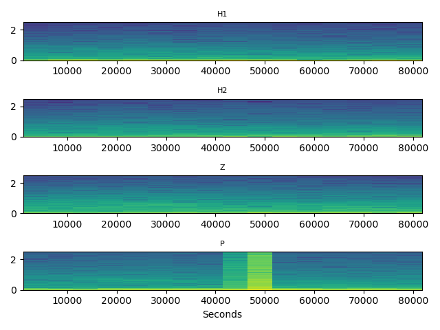
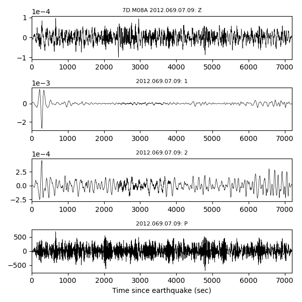
Figure 2: Daily spectrogram for the vertical (Z), horizontals (H1, H2), and pressure (P) components.
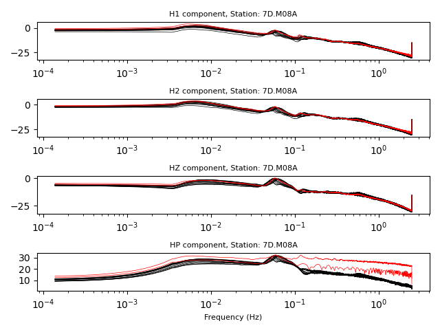
Figure 3a: Power spectral density (PSD) functions for the Z, H1, H2, and P compo- nents from a single day of data (M08A, March 4, 2012, same as in Figure 2). The left column shows PSDs for each individual window; PSDs from windows that did not pass the quality control are colored red.
Figure 3b: Daily average PSD of bad (red) and good (black) windows.
You can also choose to plot the tilt estimate for DayNoise objects. For intance, you can run:
$ atacr_daily_spectra -O --fig-tilt --tilt-freqs=0.,0.005 --start=2012-03-04 --end=2012-03-05 M08A.pkl > logfile
which will produce the figure:
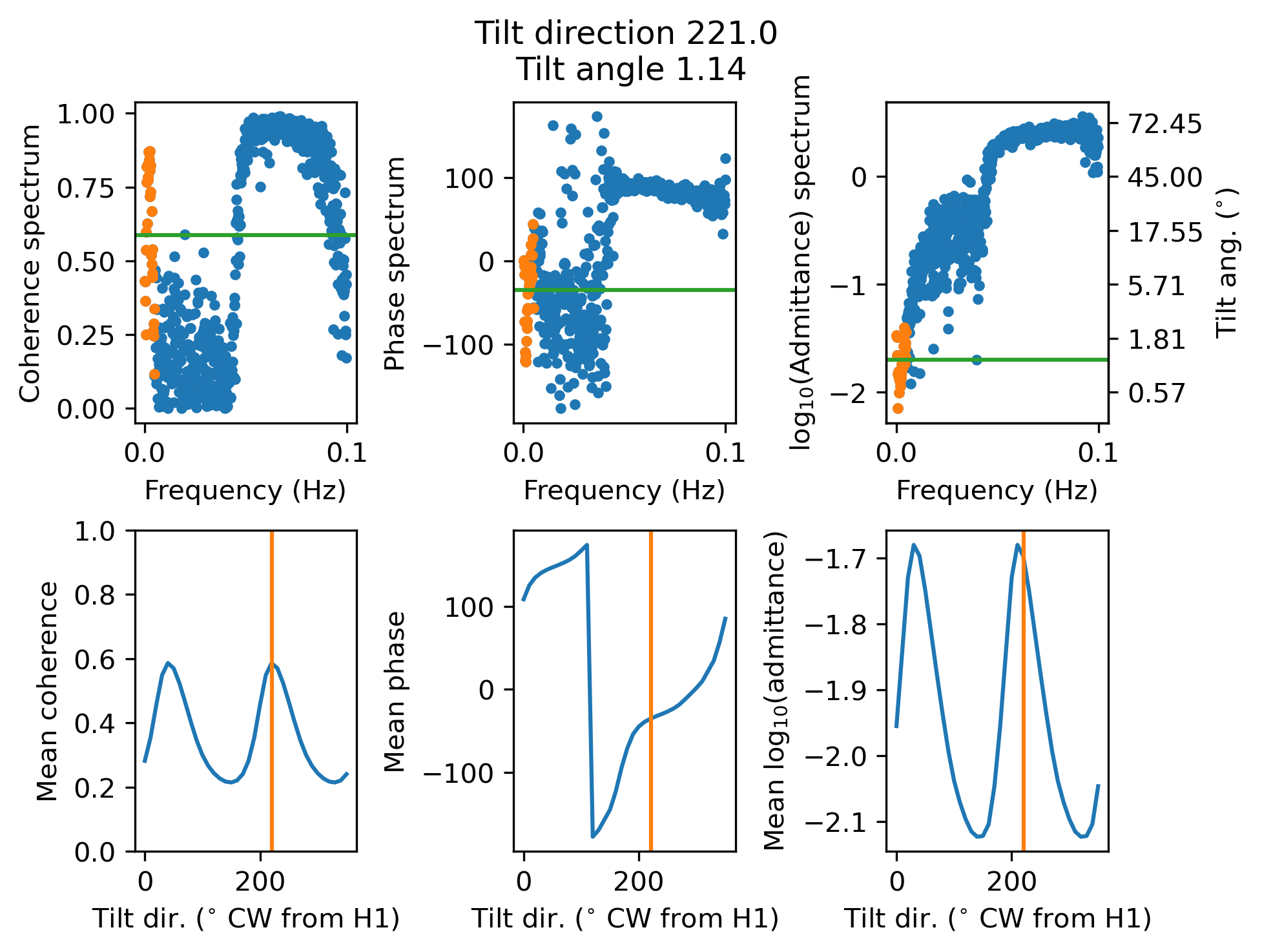
Figure 3c: Estimates of tilt direction (degrees clockwise from H1) and tilt angle. Top: coherence, phase and admittance spectra from the daily average spectra. Orange dots show the narrow bandwidth (tilt-freqs) used to calculate mean values (bottom row). The plots on the top row are shown at the tilt direction. Bottom: Mean coherence, phase and admittance as a function ot the tilt direction. The correct coherence peak is selected as the direction for which the phase is within +/- 90 degrees from 0. The admittance is used to calculate the tilt angle.
3. QC for clean station averages
Now that we have processed daily spectra for all available components, it is
possible to further average the spectra over multiple days to produce a cleaned
station average. It is still possible to specify a date range over which to
average the spectra, thus giving flexibility in the production of the station
averages. Parameter settings are similar to those used in atacr_daily_spectra
but further include the option of plotting the averaged cross-spectral properties.
To calculate a single station average for the entire month of March 2012 (and
therefore using all available data) and plot the results, we can type in a terminal:
$ atacr_clean_spectra --figQC --figAverage --figTilt --figCross M08A.pkl

###################################################################
#       _                                          _              #
#   ___| | ___  __ _ _ __      ___ _ __   ___  ___| |_ _ __ __ _  #
#  / __| |/ _ \/ _` | '_ \    / __| '_ \ / _ \/ __| __| '__/ _` | #
# | (__| |  __/ (_| | | | |   \__ \ |_) |  __/ (__| |_| | | (_| | #
#  \___|_|\___|\__,_|_| |_|___|___/ .__/ \___|\___|\__|_|  \__,_| #
#                        |_____|  |_|                             #
#                                                                 #
###################################################################


Path to AVG_STA/7D.M08A/ doesn`t exist - creating it

|===============================================|
|===============================================|
|                       M08A                    |
|===============================================|
|===============================================|
|  Station: 7D.M08A                             |
|      Channel: BH; Locations: --               |
|      Lon: -124.90; Lat:  44.12                |
|      Start time: 2011-10-20 00:00:00          |
|      End time:   2012-07-18 23:59:59          |
|-----------------------------------------------|

**********************************************************************
* Calculating noise spectra for key 7D.M08A and day 2012.061
*   -> file SPECTRA/7D.M08A/2012.061.spectra.pkl found - loading

**********************************************************************
* Calculating noise spectra for key 7D.M08A and day 2012.062
*   -> file SPECTRA/7D.M08A/2012.062.spectra.pkl found - loading

...

* Clean station spectra saved to:
*   AVG_STA/7D.M08A/2011.293-2012.200.avg_sta.pkl

* Tilt direction as function of time saved to:
*   AVG_STA/7D.M08A/2011.293-2012.200.tilt.csv
The new StaNoise object and the daily tilt directions are saved to a newly created folder called AVG_STA/7D.M08A/.
Note
If you don’t specify the options --start and --end, the object
will be saved with a filename that corresponds to the entire deployment time
of the station, but in fact the object contains the average spectra of all
daily spectra available on disk, and not necessarily the average over the
entire deployment time. We recommend using the --start and --end options
if you want to produce time-limited spectral averages (e.g., an average per week
or per month, etc.). For example:
$ atacr_clean_spectra --start=2012-03-01 --end=2012-03-08 -O M08A.pkl
Several figures are also produced, including Figures 4, 6-9.
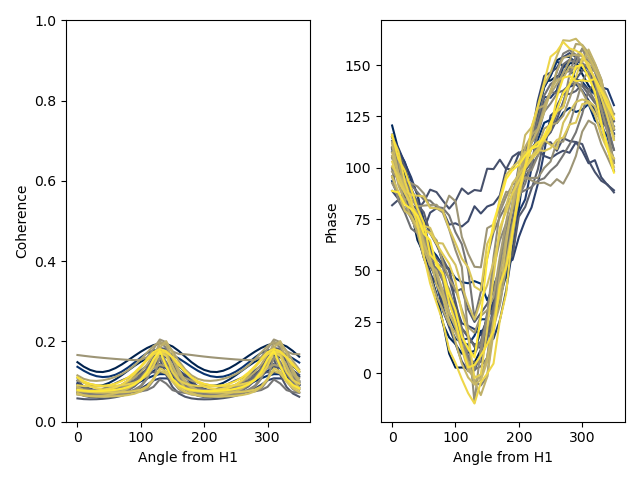
Figure 4: Tilt orientation estimates for M08A during March 2012. (Left) Coherence as a function of azimuth measured clockwise from the H1 component. (Middle) Phase as a function of the azimuth. (Right) Admittance and related tilt angle as a function of the azimuth. Dotted lines indicate estimates for “bad” days (i.e., with too few good windows). (Bottom) Tilt direction, tilt angle and maximum coherence as a function of time. Symbols marked by an “x” indicate estimates for “bad” days. The legends show the mean and 2-sigma error on the “good” estimates.
Note
In the MATLAB version of ATaCR, the “Angle from H1” (Figure 4 in the manual) corresponds to a counter-clockwise rotation of H1 and H2. Here, the angle corresponds to a clockwise rotation and the estimate is chosen to lie within +/- 90 degrees from a phase value of 0. Furthermore, we use a circular mean (as opposed to a linear mean) to calculate the phase, and consider a narrower range of tilt frequencies closer to 0 Hz, where tilt effects are most pronounced. This results in a different plot between the OBStools version and the MATLAB ATaCR version, but these differences should not affect the tilt noise removal process.
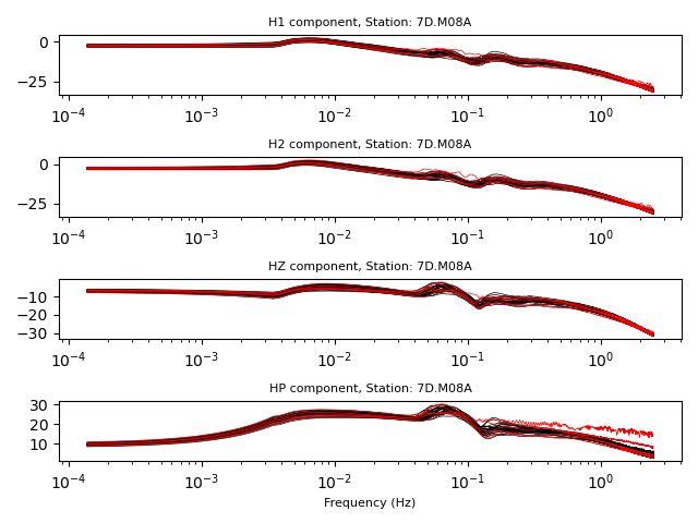
Figure 6: The daily PSDs plotted for the vertical (Z), horizontal (H1, H2), and pressure (P) components for March 2012 at station M08A. Each line is a daily PSD. Gray colors indicate days that were accepted by the second quality control step, while the red colors indicate days that were discarded.
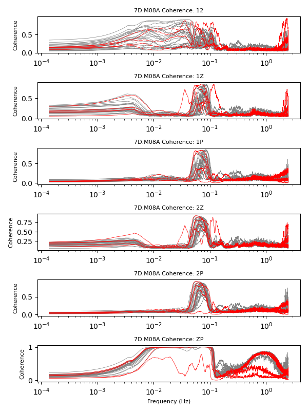
Figure 7: The daily coherences between pairs of components as indicated above each
subplot for March 2012 at station M08A (e.g. 1Z - coherence between Horizontal 1
and Vertical). Each line represents average coherence for a single day in the data
set. Gray colors indicate days that were accepted by the second quality control step,
while the red colors indicate days that were discarded. Note that some definitions
are different (e.g., ZP vs PZ) than those used in the Matlab Tutorial.
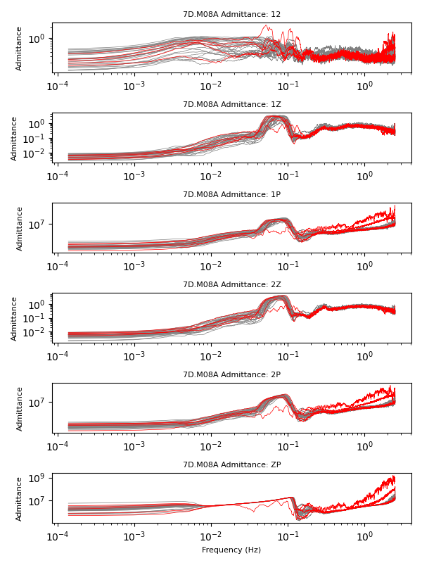
Figure 8: The daily admittances between pairs of components as indicated above
(see Figure 7) each subplot for March 2012 at station M08A. Each line is a daily
admittance. Gray colors indicate days that were accepted by the second quality
control step, while the red colors indicate days that were discarded.
Note that some definitions are different (e.g., ZP vs PZ) than those used
in the Matlab Tutorial.
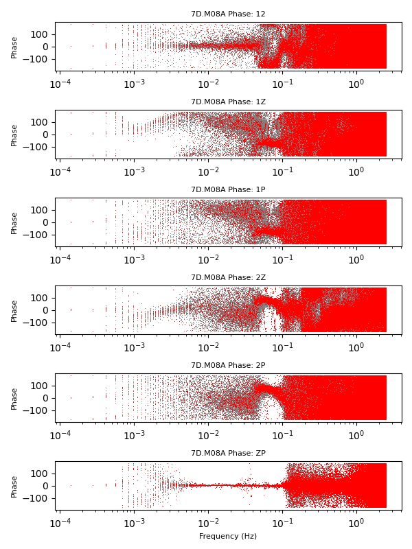
Figure 9: The daily phases between pairs of components as indicated above (see
Figure 7) each subplot for March 2012 at station M08A. Each line is a daily phase.
Gray colors indicate days that were accepted by the second quality control step,
while the red colors indicate days that were discarded. Note that some definitions
are different (e.g., ZP vs PZ) than those used in the Matlab Tutorial.
4. Transfer function calculation
Once the StaNoise objects have been produced and saved to disk, the transfer
functions across all available components can be calculated. By default the software
will calculate the ones for which the spectral averages are available.
For compliance only (i.e., only ?HZ and ?DH? components are available),
the only transfer function possible is:
ZP
For tilt only (i.e., all of ?HZ,1,2 components are available, but not ?DH),
the transfer functions are:
Z1Z2-1
For both tilt and compliance (i.e., all four components are available), the following transfer functions are possible:
Z1Z2-1ZPZP-21
If you are using a DayNoise object to calculate the transfer functions,
the following may also be possible (if all components are available):
ZHZP-H
In this example we calculate all available transfer functions for all available data. In this case we do not need to specify any option and type in a terminal:
$ atacr_transfer_functions M08A.pkl

#######################################################################################
#  _                        __             __                  _   _                  #
# | |_ _ __ __ _ _ __  ___ / _| ___ _ __  / _|_   _ _ __   ___| |_(_) ___  _ __  ___  #
# | __| '__/ _` | '_ \/ __| |_ / _ \ '__|| |_| | | | '_ \ / __| __| |/ _ \| '_ \/ __| #
# | |_| | | (_| | | | \__ \  _|  __/ |   |  _| |_| | | | | (__| |_| | (_) | | | \__ \ #
#  \__|_|  \__,_|_| |_|___/_|  \___|_|___|_|  \__,_|_| |_|\___|\__|_|\___/|_| |_|___/ #
#                                   |_____|                                           #
#                                                                                     #
#######################################################################################


Path to TF_STA/7D.M08A/ doesn't exist - creating it

|===============================================|
|===============================================|
|                       M08A                    |
|===============================================|
|===============================================|
|  Station: 7D.M08A                             |
|      Channel: BH; Locations: --               |
|      Lon: -124.90; Lat:  44.12                |
|      Start time: 2011-10-20 00:00:00          |
|      End time:   2012-07-18 23:59:59          |
|-----------------------------------------------|

**********************************************************************
* Calculating transfer functions for key 7D.M08A and day 2012.088

**********************************************************************
* Calculating transfer functions for key 7D.M08A and day 2012.075

...

**********************************************************************
* Calculating transfer functions for key 7D.M08A and range 2011.293-2012.200.
Note how the DayNoise objects are read randomly from disk, followed by the
StaNoise object. The result is a TFNoise object that is saved to a newly
created folder called TF_STA/7D.M08A/.
We can produce Figure 10 by re-running the previous command with the options
-O --figTF.
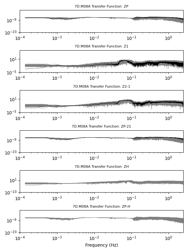
Figure 10: Transfer function amplitudes for the component combinations of interest, as indicated in the title of each subplot. This example is for the month of March 2012 for station M08A. The daily transfer functions are shown in grey and the average calculated for the whole month is shown in black.
5. Download earthquake data
Now we need to download the earthquake data, for which we wish to
clean the vertical component using the transfer functions just calculated.
This script atacr_download_event is very similar to atacr_download_data,
with the addition of the Event and Geometry Settings.
Warning
Be careful with the Frequency Settings, as these values need to be exactly
the same as those used in atacr_download_data, but won’t be checked
against.
To download the seismograms that recorded the March 9, 2012, magnitude 6.6 Vanuatu earthquake (be conservative with the options), type in a terminal:
$ atacr_download_event --min-mag=6.3 --max-mag=6.7 --start=2012-03-08 --end=2012-03-10 M08A.pkl

###############################################################################
#      _                     _                 _                         _    #
#   __| | _____      ___ __ | | ___   __ _  __| |    _____   _____ _ __ | |_  #
#  / _` |/ _ \ \ /\ / / '_ \| |/ _ \ / _` |/ _` |   / _ \ \ / / _ \ '_ \| __| #
# | (_| | (_) \ V  V /| | | | | (_) | (_| | (_| |  |  __/\ V /  __/ | | | |_  #
#  \__,_|\___/ \_/\_/ |_| |_|_|\___/ \__,_|\__,_|___\___| \_/ \___|_| |_|\__| #
#                                              |_____|                        #
#                                                                             #
###############################################################################


Path to EVENTS/7D.M08A doesn't exist - creating it

|===============================================|
|===============================================|
|                       M08A                    |
|===============================================|
|===============================================|
|  Station: 7D.M08A                             |
|      Channel: BH; Locations: --               |
|      Lon: -124.90; Lat:  44.12                |
|      Start time: 2011-10-20 23:50:00          |
|      End time:   2012-07-18 23:06:00          |
|-----------------------------------------------|
| Searching Possible events:                    |
|   Start: 2012-03-08 00:00:00                  |
|   End:   2012-03-10 00:00:00                  |
|   Mag:   6.3 - 6.7                            |
| ...                                           |
|  Found     1 possible events                  |

************************************************************
* #(1/1):  20120309_070953
*   Origin Time: 2012-03-09 07:09:53
*   Lat: -19.22; Lon:  169.75
*   Dep:  33.70; Mag: 6.6
*   Dist: 9651.91 km;   86.80 deg
*   2012.069.07.09*.SAC
*   -> Downloading BH1 data...
*      ...done
*   -> Downloading BH2 data...
*      ...done
*   -> Downloading BHZ data...
*      ...done
*   -> Downloading ?DH data...
*      ...done
* Start times are not all close to true start:
*   BH1 2012-03-09T07:09:53.336000Z 2012-03-09T09:09:52.336000Z
*   BH2 2012-03-09T07:09:53.336000Z 2012-03-09T09:09:52.336000Z
*   BHZ 2012-03-09T07:09:53.336000Z 2012-03-09T09:09:52.336000Z
*   BDH 2012-03-09T07:09:53.336000Z 2012-03-09T09:09:52.336000Z
*   True start: 2012-03-09T07:09:53.320000Z
* -> Shifting traces to true start
*   -> Removing responses - Seismic data
 WARNING: FIR normalized: sum[coef]=9.767192E-01;
 WARNING: FIR normalized: sum[coef]=9.767192E-01;
 WARNING: FIR normalized: sum[coef]=9.767192E-01;
*   -> Removing responses - Pressure data
 WARNING: FIR normalized: sum[coef]=9.767192E-01;
The data are stored as an EventStream object, saved to disk in the
newly created folder EVENTS/7D.M08A/.
6. Correct/clean earthquake data
The final step in the analysis is the application of the transfer functions
to the raw earthquake seismograms to clean up the vertical component.
Once again, the default settings can be used. The corrected seismograms will
be saved to disk in a new folder called EVENTS/7D.M08A/CORRECTED. To make
the final Figures 11 and 12, specify the --figRaw and --figClean options:
$ atacr_correct_event --figRaw --figClean M08A.pkl

##################################################################
#                               _                           _    #
#   ___ ___  _ __ _ __ ___  ___| |_     _____   _____ _ __ | |_  #
#  / __/ _ \| '__| '__/ _ \/ __| __|   / _ \ \ / / _ \ '_ \| __| #
# | (_| (_) | |  | | |  __/ (__| |_   |  __/\ V /  __/ | | | |_  #
#  \___\___/|_|  |_|  \___|\___|\__|___\___| \_/ \___|_| |_|\__| #
#                                 |_____|                        #
#                                                                #
##################################################################


|===============================================|
|===============================================|
|                       M08A                    |
|===============================================|
|===============================================|
|  Station: 7D.M08A                             |
|      Channel: BH; Locations: --               |
|      Lon: -124.90; Lat:  44.12                |
|      Start time: 2011-10-20 23:50:00          |
|      End time:   2012-07-18 23:06:00          |
|-----------------------------------------------|
TF_STA/7D.M08A/2011.293-2012.200.transfunc.pkl file found - applying transfer functions
TF_STA/7D.M08A/2012.069.transfunc.pkl file found - applying transfer functions
Results are saved both as updated EventStream objects and as .SAC files that
now contain the corrected vertical components.
Note
The EventStream object contains the corrected traces in the attribute
correct, which is a dictionary. If you wish to extract the corrected
vertical seismogram obtained from the ZP transfer function, with a corresponding
key 'ZP', you can do this by loading the .pkl file and typing:
>>> # First load the EventStream object
>>> import pickle as pkl
>>> evstream = pkl.load(open('2012.069.transfunc.pkl', 'rb'))
>>> # Extract the 'ZP' corrected seismogram
>>> corrected = evstream.correct['ZP']
You can check which transfer functions should be available based on the number of
components in the EventStream object from the attribute:
>>> print(evstream.ev_list)
Note that the corrected seismogram will only be available if the corresponding transfer function has been calculated previously and applied during the correction.
Figures 11 and 12 should look like:
Figure 11: Event time series for the vertical (Z), horizontal 1 (H1), horizontal 2 (H2), and pressure (P) components. No corrections have been applied. The data is for station M08A for the Mw 6.6 earthquake that occurred near Vanuatu on March 9, 2012 and has been bandpass filtered from 10 - 150 s.
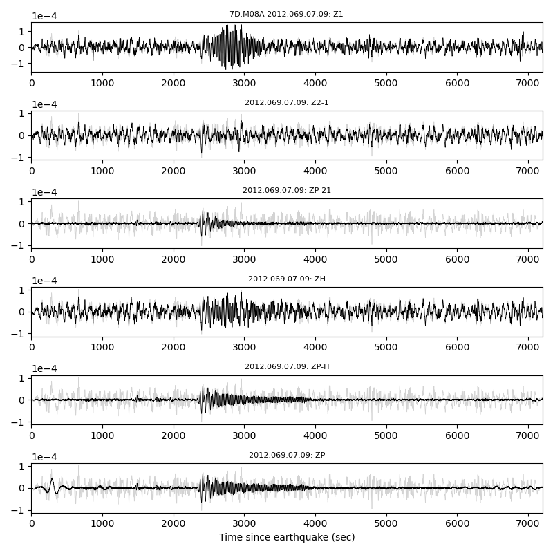
Figure 12a: Event time series for the vertical (Z) components after each of the transfer functions of interest have been applied. The corrections are specified in the titles of each subplot. The data is for station M08A for the Mw 6.6 earthquake that occurred near Vanuatu on March 9, 2012 (same as Figure 11) and has been bandpass filtered from 10 - 150 s. Traces in grey show the original (raw, un-corrected) vertical component.
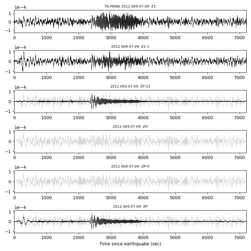
Figure 12b: Same as Figure 12a but using the station averaged transfer functions. In this
case the ZH and ZP-H transfer functions are not available.